
In the mid 20th century, the college board became curious about what the distribution of SAT scores would be if ALL American 17-year-olds took the SAT, not just the college bound elite. One reason for this curiosity was the average score of people who actually took the SAT started falling in the 1960s, especially the verbal scores, so people wanted to know whether this was simply because less elite kids were applying to college, or if teens in general were being dumbed down (see chart from Herrnstein & Murray, 1994; page 425):

This is discussed in the book The Bell Curve:


What they found was that the decline was just an artifact of the SAT population becoming more inclusive. When you look at nationally representative samples, not only was there no decline, but there was actually a very small Flynn effect.
I was especially interested in seeing these national norms because the SAT has long been considered a good proxy for IQ, but unlike IQ tests which are normed to have a mean and standard deviation of 100 and 15 in the general U.S. population, the verbal and math subscales of the pre-1995 SAT were both normed to have a mean and SD of 500 and 100 respectively and with respect to the 1940s SAT taking population (not the general U.S. population). The chart above tells us how the average U.S. 17-year-old (IQ 100) would have scored on the SAT from 1950s to the 1980s, but to fill in the rest of the IQ distribution, we need to know the standard deviations.
Thanks to Charles Murray, I was able to find the SDs for the 1980s and I had already found the SDs for the 1970s.
What about the 1960s? I recently discovered this data from the 1960 norming study:
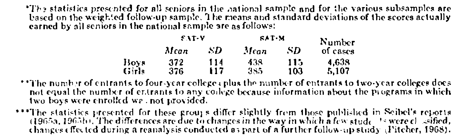
Unfortunately the data is stratified by sex (if they tried that today they’d need categories for non-binary, gender fluid, two spirit). Well to determine the mean of the entire cohort, we take the weighted average (52% female) so verbal mean = 0.52(376) + 0.48(372) = 374. Math mean = 0.52(385) + 0.48(438) = 410.
These figures perfectly match the 1960 figures from The Bell Curve book which I showed at the top of this article so I must have done something right!
Now combining the SDs of men and women is much more difficult (even chat GPT can’t do it!). You can’t just average them because the size of the combined SD is not just a function of the two SDs, but how far apart the two means are. Of course if we assume the male, female, and sex-combined distributions are all perfectly Gaussian it’s kind of easy to estimate, but estimating is very different from actually calculating (and when men and women are too far apart, it’s probably impossible for all three distributions to be Gaussian.
To determine the sex-combined SD we must first determine the Sum of Squares:
Sum of Squares = female n*(female sd^2 + female mean^2) + male n*(male sd^2 + male mean^2)
And then:
sex combined standard deviation is SQRT(Sum of Squares / sex combined N – sex combined mean^2)
And so for 1960, the sex-combined mean and SD for verbal and math respectively were 374; 116 and 410; 114 respectively.
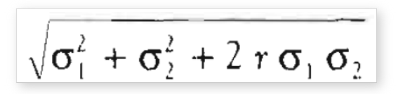
To determine the sex-combined composite mean we just add the verbal + math mean = 784, and assuming the 0.67 correlation between verbal and math and the below formula (Herrnstein & Murray, 1994, page 779), the composite SD was 210.

Guys I just realised something. I don’t think Melo accepts HBD lol. Hahahaha.
LMAO
You just realized this?
What a dumbass!
Probably because you’ve literally said you accept HBD before, so…
Jesus christ. When everyone here accepts that jews run everything (even Bruno lol), and youre the only guy who says its offensive or hurts your feelings to know it, then maybe look at your conditioning. All the high IQ people know this as a fact of HBD. Melo is rejecting jewsdidit because…CNN told him it was a stereotype….great carpenter reasoning Melo. listen to the jews about why they have no power. Hahaha.
Trump is going to beat Kamala by at least 5 points. If they kept worrying they couldn’t put Biden out in front of people, that problem is even worse with a schizo like Kamala. Kamala makes Loaded sound like Cicero.
Just watch the videos where shes asked to speak off script. Its comical.
The other ‘sad’ fact is that a good chunk of white men will never vote for a black woman. A good chunk of latino men won’t either.
But Kamilla has the best of both Worlds in that she’s just black enough to be considered black in the U.S., yet still Caucasoid enough to remind you of your suburban mom.
And while she’s not smart by World Leader standards, she’s dumb in a charismatic way, like the fun ditzy co-worker who is always laughing at her own incompetence. Trump is already showing signs of being scared.
“she’s dumb in a charismatic way, like the fun ditzy co-worker who is always laughing at her own incompetence. Trump is already showing signs of being scared.”
EXACTLY!
I didn’t know much about her before she started campaigning, but now my TikTok is being overrun with memes and videos on her.
She’s weirdly charismatic. The right-wing media would have you convinced she’s like Hilary…but she doesn’t act like her at all. She laughs a lot and has energy. If the ads start to contrast that with a grumpy and serious Trump, people will start to gravitate towards her.
She’s energized dems and started breaking donation records. We might actually have this. BUT, this could also just be a honeymoon phase and soon everything will go back to the normal programming.
?? Trump was laughing at her when she became the favourite. He called her pathetic. Its on video in his golf cart.
Trump will totally destroy Kamala in a debate. Kamala will do grifter ‘sexism’ and ‘racism’ arguments and Trump will just stand on it.
Youre talking about a top 1% social IQ person vs an AA hire person that can barely finish a sentence without a script.
All AA hires are total clowns like Afro and these other diversity people.
“1% social IQ person”
LOL
peepee once again admits she is a black woman.
Good ol Melo. Still living in 1965. Keep it strong my brother!
Black POWAH. Black POWAH.
Yes, my brother. Soon our Jewish masters will eradicate the evil whitey and all of our wives and and daughters will be filled to the brim with black baby gravy.
You realise blacks would beat the living crap out of you even if you kiss their asses?
I’ve lived around blacks, they’re not that bad lmao.
I also think Trump would beat Obama in a debate even though Obama is much more sophisticated and has objectively better policies.
Its called SOCIAL INTELLIGENCE. Look it up Puppy. Its more important than academic intelligence for human survival.
LOL! What the hell do you know about survival? The government literally supports you because otherwise you’d starve to death on the streets.
Its simply a fact that I’m more R selected than you. You wouldn’t be viable in places like Africa or these other hellholes where people stand on peoples heads while they sleep.
r selected (the r is always lower case even at the start of sentence) means one can’t survive which is why they compensate for low survival rates with high birth rates.
Ok, you need Marsha to explain Rushton’s book to you.
I would vote Trump over Harris.
I Would have gone for Biden over Trump, but a schizo idiot AA hire is a total disaster. Shes just a complete puppet for you-know-who. At least Trump would actually be the person you vote for.
I know how Harris became a politician. She slept with guys like Willie Brown and those other black ‘statesmen’ in californian politics to get the backing.
I’m not sure that disqualifies her. Hilary is a psychopath and obviously Nikki Haley is even more of a jew puppet. So of the women, Harris is the best of a horrible bunch.
Kamala looks like she gives good head.
Coconut Party ftw!
Sorry, the best woman candidate was an is Marianne Williamson. The jew.
Harris will win 20% of the white male vote lol. And half of that will be gay men.
yes. pill doesn’t get why leftists would prefer trump and why they’d never vote for biden or karmelo.
melo and peepee are just low IQ evil racists, not leftists, so they don’t unnuhstan either.
hint: part of the reason is the same reason berezovsky supported the communist party vs putin.
another hint: part of the reason is the same reason the anti-war pipo protested the DNC in chicago in ’68 but didn’t protest the RNC.
the Doors even have a song about it. let’s hope for a repeat in august. this time it’s not vietnam. it’s gaza.
I don’t need any hints; my IQ is FIFTY POINTS above your level. Because Trump challenges the system, while Democrats work within it.
Puppy doesn’t get it as usual. The argument is the dems need to be wiped out to start over. From this point of view Kamala is an excellent choice. It would be even better if they chose a random homeless person. Its the same argument Jimmy Dore made in 2016. You select something abhorrent to the point that neocons have to change their policies on the dem side to be a bit more appealing to real people, presuming the republicans keep running populists.
Cenk likes to joke the Biden keeps bragging that his greatest achievement is expanding NATO. Its not very funny because Biden truly believes that is his greatest achievement even if nobody cares. The point Cenk doesn’t get is that Biden cares about it because that what the neocons in Washington care about. The couldn’t give a shit about the minimum wage or the budget or healthcare or literally any other issue outside of using the US army to enact lebensraum.
Puppy doesn’t get it as usual. The argument is the dems need to be wiped out to start over.
No the SYSTEM needs to be wiped out to start over. Your answer would apply to any Republican, not Trump only.
peepee says trump is the mossad candidate.
but then how can he be anti-neocon?
either:
2. the iraq war was NOT just about israel. OR
3. peepee is a self-contradicting muslim narcissist who thinks it’s always about her.
DUH CHROOF: trump combines zionism with anti-neocon-ism. deal with it. because pure zionism gets him lots of jewish $$$ without having to hurt americans. (((wokeism))) and foreign forever wars are WAY worse for americans than moving the US embassy to jerusalem. like WAY!
I thought Trump was hugging the neocons to keep them from starting wars too. But actually trump was often many times close to invading Iran. He made the neocon John Bolton his Sec of State. He had to be talked out of the invasion of Iran by staffers.
Look, theres no 3d chess. Trump isn’t very bright academically. But socially he knows he has to kiss jewish ass. I think if hes president theres a 50-50 chance Iran gets invaded.
But with Hilary, De Santis, Jeb or Nikki Haley its more like 90%. If Adelson orders it, it will happen.
peepee says trump is the mossad candidate.
but then how can he be anti-neocon?
Because while Trump is great for Israel, he’s bad for U.S. Jews. Mossad mostly cares about the former while the U.S. neocons care about both; hence they disagree on Trump.
Kamala presumably will have similar policies to Biden but be beholden to ashkenazim maybe even more so than Biden. All black politicians with the sole exception of Barack Obama follow jew orders to the letter. You might even see Kamala send US troops to fight Hamas.
In my lifetime, every single diversity political candidate represented the establishment in every country you want to name. Going back to Thatcher. Its a cute trick they use that fools people like Melo and Puppy.
Woman. Black. Gay. Trans. Latino. etc. They literally take these people off the side of the street. Wash them. Put them in nice clothes and teach them what to say.
Again, the sole exception to this general rule of politics is Barack Obama who is a genuinely strange case of someone who wanted to do good.
Going back to Thatcher. Its a cute trick they use that fools people like Melo and Puppy.
Actually I’ve only praised black media figures & these are generally WAY more subversive than their white peers.
Blacks parrot the establishment line on all issues and especially black issues.
When Kanye spoke against the elites, they literally marched every black celebrity this side of Iran into a press conference to denounce Kanye.
When Kanye spoke against the elites, they literally marched every black celebrity this side of Iran into a press conference to denounce Kanye.
Complete nonsense. Tons of black celebs & politicians have at one point or another been under attack for saying something the establishment defined as anti-Semitic. AIPAC just went on a wild spending spree defeating Jamal Bowman.
Candace Owens just got fired from Ben Shapiro’s company for criticizing Israel & its supporters constantly, non-stop, and still is.
Brianna Joy Gray just got fired from The Hill for not supporting Israel. Mark Lamont Hill got fired from CNN for defending Palestinians.
Congress woman Cynthia McKinney linked 9/11 to Zionists.
Nina Turner lost an election for opposing Israel.
Louis Farakhan, one of the most influential black leaders of all time, constantly criticizes zionists.
Jesse Jackson described new York using anti-semetic slur T
he top dog of black politics Al Sharpton was called anti-semetic.
Ilhan Omar constantly opposes Israel.
Former Harvard Professor Cornell West is one of the loudest critics of Israel.
The first black president of Harvard just got fired for not being pro-Israel enough. Even Michael Jackson blamed the fall of his career on Jews.
Obama & Kanye are the rule, not the exception.
Ok, I meant the establishment blacks like Clyburn, Jay Z, Clarence Thomas, and so on.
Yeah youre right. In the UK, the labour party basically purged a bunch of black politicians for not supporting israel.
Yeah its bizarre the 2 biggest anti establishment candidates are Williamson and Bernie and both are ashkenazim.
I don’t want to joke, but Jimmy would literally say they were pretend opposition.
hegel on steroids.
in a two party system…
what if your party is gay and retarded? like steals the nomination from bernie?
what do you do?
and then sean o’brien gives speech at GOP.
it is a FACT! that under trump’s admin wages went up FASTER at the low end than the high.
did that trend continue with biden?
the dems are the FAKE LEFT.
the GOP is the FAKE RIGHT.
which has become even more FAKE with trump.
AND this is a good thing!
trump has destroyed the old GOP and moved the GOP to the LEFT.
melo: but trump is evil and orange.
mugabe: but he got ‘er done!
reminds me of that nobel laureate “racist”‘s Playboy interview…
he was axed “so what’s a smart person? what’s smart?”
he said:
smart pipo are better getting things done.
https://www.playboy.com/magazine/articles/1980/08/playboy-interview-william-shockley
Yeah Mugabe’s analysis is correct. Trump actually pushed the republican party to the left, not the right.
They (ie Goldman Sachs) rigged it against Bernie plain and simple. The Mass. primary, the Nevada one. On and On you get tiny vote margins. Evidence of a rigging.
The south korean election was the same. 0.1% winning margin. Means its rigged.
I can’t remember where I first read that. But basically the political analyst (ie a real one, not puppy) made the rule that said whenever a vote is very tight and the establishment candidate wins by 0.1% of the vote, its rigged.
You can’t manufacture millions of fake votes. But you can a few thousand, or in Bernie’s case, a few hundred.
“Trump actually pushed the republican party to the left, not the right.”
Lol. Autism confirmed.
indeed. melo confirms his autism and low IQ and racism.
sad.
It depends on who you believe is the heart of (the actually good part of) the US. Trump appealed to those people a lot more than previous Republicans.
Obviously Trump was a populist. You don’t become a “populist” by not appealing to the majority of the population. That’s one of the major definitions of being “left-wing”.
(((mind control))) works on pill and lurker personalities. sad.
“populist” is a pejorative like “demogogue”. why? what does it really mean? it means “the pipo are too stupid to vote but we (the meat puppets of the elite) loves ourselves some democracy.” it’s a self contradictory pejorative that can only be used by meat puppets.
democracy = populism = demogogue = peepee is an old version of chatGPT = sad.
“peepee and melo = low IQ racists = meat puppets = sad.“
Meat Puppets had some good songs though.
Also, I don’t know why Melo is annoyed by right-wingers and their “overly simplistic worldviews” while literally labeling them as simpletons and idiots just because he doesn’t agree with them because he has his own simplification of the world where if you explicitly hold some simplistic beliefs you are automatically wrong and unnecessary for humanity’s progress (ironic! isn’t it?), even though it is obvious what harm overly liberal and open-minded worldviews are doing to the West without a steadfast and stubborn belief in some tradition and keep society functioning and on the right path.
Once again Juden Peterstein shows greater moral understanding of the proper meta-ordering of the symbiotic relationship between chaos and order…
jews read Melo’s comments and rub their hands while eating a delicious matzoh ball soup!”peepee and melo = low IQ racists = meat puppets = sad.“
Meat Puppets had some good songs though.
[error redacted by pp, 2024-07-23]
Social Intelligence vs Quant Intelligence
Mostly it is just about “motion” vs “static shapes”
That is why emotional intelligence exists.
You understand how people move dynamically.
Where as objects are statically controlled.
Yes, quant intelligence is a number of parts can be high.
But social is about many things in motion as in people.
More people see kamala as a people person than trump.
Trump can order people about, but Kamala listens.
That is the male-female dichotomy.
–
Male social intelligence then is not female social intelligence.
Males can “get things done” but only if there decisions are corrects most of the time for people to follow them.
Females get people to work together so their intuition happens to be about knowing who is least likely to be ego driven and make big mistakes.
Hillary was a psychopath, so Trump took advantage of that.
Kamala being with biden so long will not be as easy to defeat.
The SYSTEM as pumpkin puts it, is more female oriented, people don’t want it to be reformatted, They want the three branches of government to remain in balance of powers.
The guy I said was my stepfather told me this christmas the democrat’s would put hunter biden in charge as dictator creating a dynasty of bidens, if joe biden won. He lacks female social intelligence.
Great observation! I’ll be thinking about that.
Good point, this is very similar to the idea that PP espoused of “ironic autism” or having your autistic obsession being people and social interaction.
Another great point. I want to stab my eyes whenever I see some TERF talk about how transwomen in women’s sports is “patriarchy”. The patriarchy is the patriarchy even when it’s not the patriarchy as long as biological males somehow get an advantage over biological females… in a literal fair competition using only one’s biological body. Lol. Just shows you how retarded we’ve gotten.
“the system” is just pipo peepee. trump’s plan is to replace the evil retarded pipo with his pipo. his plan is not to make a new constitution.
peepee’s low IQ is sad and hilarious.
member how rr hates if you reference wikipeida
Most of if not all of the 2025 project is about restructuring the executive branch to give more power to the president.
lurker says they at the top have 100 plans
well they do but not all agree so it changes
righties believe climate change is a hoax so will get rid of several science org of the gov – and other things that require more president power
because last time trump had not enough power
political people seek power so trump is just the proxy
and those at the top see trump as a means to do stuff/change things in the gov
not all bad but heh, gov don’t want that
He might as well have changed the constitution. He undermined America’s trust in elections and the fourth estate. Love him or hate him, he was one of the most consequential presidents of all time.
that was the wrong clip. sorry.
https://www.youtube.com/watch?v=NbHPTfG1YjM
yes, working class people matter
but then some if not most religious don’t like mug because homosexual
it is weird thing to be so pro-working class yet hate science and sheet
I know trump don’t buy that science is wrong, he still must be populist.
don’t get me wrong
rr disbelieves evolution so left are not off the hook
melo personality: calling kamala karmelo is hate speech.
mugabe: true. i hate karmelo. but because she’s a sociopath. not because she’s a dugla. everyone hates her. she’s evil.
melo: hating any dugla is racisss. hating any jew is antisemitism. hating every wypipo is anti-racism.
mugabe: (((mind control))) works on filipinos. sad.
Why does Mugabe keep commenting when he’s irrelevant?
Alcoholic-induced psychosis is sad.
i am irrelevant to curing your autism and mental retardation melo. but this blog isn’t here for that either.
Accelerationist’s solution to a broken finger is to cut off the whole arm.
That’s your solution to inequality though. Try to eliminate all inequality through whatever means are necessary even if they are obviously worse than whatever problems your “solutions” aimed to solve.
Haven’t you paid attention to what has happened to this country under increasing liberal policies? As a liberal, you constantly get your way in the country, and when you don’t, it’s not because of wypipo but because of neocons aiming policy towards their own interests in world dominion. The only time liberals haven’t gotten their way is with useless distracting BS like Roe v Wade being overturned. Do you bank bailouts and sky-high inflation are “right-wing”? You’ve basically labeled everything you don’t like as right-wing.
You may claim that the progressive nature of our society is due to fearless half-filipino men who have paved the way with their blood, sweat, and tears ever since they came to North America to found this country in 1976, but in reality, you could say the so-called “patriarchy’ is also the result of the fierce toil of males, or that the consistent extreme wealth gap of global bankers and the rest of humanity is simply a testament to their stunning and brave will to fight and eliminate the competition.
We need unity:
Trump/Kamala 2024
Lurker bank bailouts aren’t liberal or conservative. They’re neoliberal. George Bush and Hank Paulson was literally dancing when he got TARP through and all the bankers kept their bullshit bonuses.
Neoliberalism is basically corruption masquerading as an ideology.
When I was a banker I 100% accepted the bonus restrictions and the ban on entertainment expenses. I knew the whole thing was rotten.
The had to nationalise the bank I was working for. It cost the taxpayer billions.
I’ve been a banker and regulator and know both sides of the argument and generally the regulator is 80% of the time correct.
You could argue most banks should be state utilities like in China or India.
it’s NOT accelerationism dumbass! LITERALLY retarded person!
mugabe: suppose trump instead of making america great again makes america brazil and has a dirty war against melo and his ilk, an operation condor stateside.
melo: then would you admit you’re wrong?
mugabe: no melo. you have autism. the democrat party can’t be reformed. it’s totally stuck at what in the rest of the rich world would be correctly called the far right. it is to the right of the british conservative party and far to the right of FN and AfD etc.. but because you’re a mentally retarded and autistic racist you confuse economic issues with idpol. in the two party system where one party is 100% stuck the only thing one can do is hope the second party unsticks it, ala berezovsky supporting the commies.
melo: hahaha! you’re so dumb you don’t even watch CNN.
mugabe: sad!
This is why Mugabe is dumb.
Trump is proof that parties CAN change!
Democrats are right-wing and socially progressive.
Republicans are right-wing and socially conservative.
OF COURSE, I will pick the one that gives me more social freedom.
There is room for discussion on whether social conservatism is actually good for society, but you and Lurker are not the people to have that discussion with because you’re bad-faith actors.
Lurker, mainly because he’s dumb and racist, and you, mainly because you’re racist and an alcoholic crybaby. You are the definition of complacency.
pp: “1.55 is just a ratio; we don’t know what the mean and SD are so you can’t estimate the rarity.”
–
mental age = iq (age / emotional age)
27.4 = 1.18 * (36 / 1.55)
simpler
All Puppy and Anime do is post equations. Its like they’re a trolling.
Melo and RR are out of their depth here. Exactly what you’d imagine if you threw a fitness bro and carpenter into a high IQ comment section. Even Anime understands it better.
Ultimately the USA is heading for a serious crisis no matter who wins because of the classic marxist analysis. You have a tiny elite that control 70% of the wealth and the judges/politicans/regulators and it just so happens most of this elite are another race.
Marx doesn’t really talk about the racial aspect in an elite.
Anyways, the crisis can only be resolved by geeing up aggregate demand through (a) colonialism (b) authoritarianism.
I predict you will start to see elites talking about how free speech needs to be ‘regulated’ or how the right to protest or organise needs to be curtailed. You will start see ‘anti terrorism’ laws broadend.
The fundamental financial problem is the USA is going bankrupt and the elites won’t pay taxes to solve the issue. So either the pensions go, or the elites stop sending money to the Caymans.
These cycles will keep continuing in every country.
I was looking at Thailand and how their aristocracy is basically just a more in your face version of America but the end result is also revolution.
I truly believe in Winston’s aphorism that eventually the proles will wake up. Theres a gigantic populist mood in every single Western country after 50 years of neoliberalism.
technically the US can’t go bankrupt because its debt is in its own currency.
but it can suffer hyperinflation if it is forced to monetize its debt.
and as bad as the national debt is in the US it is by some measures worse in japan and italy.
so why is the USD still so strong? why is GDP PPP so much higher than GDP nominal in almost every country?
GDP at PPP is 10th in the world even though you have the worlds highest oil exports and as you say plenty of natural resources and land.
USA living standards for the bottom 90% have declined since the 60s.
i know hebrew is your native language but you didn’t unnuhstan my comment.
re-read it and admit you’re an israeli.
The neocons are the elite of the elite. Whereas Koch, Mellon and these other aristocrats are there for the economics. The neocons are there for social engineering en masse.
I was thinking about the example of China under Mongolian rule or Latin America under Spaniard rule.
The neocons will try to talk back control of the system via the democrat party. The republican party is lost. Thank you trump.
If you turn on MSNBC 50% of the hosts are former Bush administration people lol.
Trump nephew reveals Uncle Donald’s racist outburst in new book | Books | The Guardian
This actually makes me like Trump even more. Great social IQ. Top 1%.
Being a racist is a U shape curve. IQ on X axis. Racism on Y.
Every single top scientist or genius without autism is a secret or open racist.
The research I’ve seen suggests racism against blacks shows low IQ but racism against Jews shows high IQ.
I suspect this is just a function of the larger correlation between left-wing views and IQ.
High IQ have more compassion & moral reasoning and thus have compassion for underdogs (blacks, the poor, women, gays, Palestinians, the environment, wildlife) while low IQ people are more psychopathic and less morally developed and thus are useful idiots for the powerful (Billionaires, corporations, Jews, whites, America, Israel).
And while it’s possible to find high IQ whites who hate blacks, they typically hate Jews more and while it’s possible to find low IQ whites who hate Jews, they typically hate blacks more.
It’s just a form of noblesse oblige. Of course if blacks continue to gain power and Jews continue to lose it, we could see a reversal, with high IQ people hating blacks and low IQ people hating Jews.
Every single high IQ person is familiar with the crime pattern. I have never in my whole life heard of a high IQ neurotypical person living among blacks in any country.
What Trump said above shows high social IQ. He immediately knew the blacks knifed his car without any evidence. Very high top 1% social IQ.
This was the 1970s before we had 50 years of crime data. Back then data collection was primitive. He knew it from observing people.
Trump was almost born to be a politician.
He also accused a bunch of innocent blacks of raping the central park jogger
He was right. She was raped but by other blacks.
but not the blacks he blamed
like james watson. but his “racism” was based on personal experience.
the problem is “racism” has become a purely ideological term of neoliberalism, the reigning ideology. so you have to say exactly what you mean by it.
and in that case it’s not U shaped.
by one definition “racism” increases from dumbest to smartest.
by another it decreases.
If you look at every single Ganzir, Anime, Bruno comment in the past 7 years on this HBD blog, not 1 criticism of blacks behaviour or IQ. Its literally impossible for an autistic person to have disgust towards a black.
It’s true that autistics are less likely to be racist, but ironically they’re probably more likely to be HBD. What they lack in disgust they makeup for in non-conformity and unintentional insensitivity.
(((commenters))) like pill and sailer are on a mission to deflect attention from (((themselves))) and toward whatever supposed black dysfunction.
“Supposed” black dysfunction wtf. Blacks are without doubt the most outrageous humans on the planet. 90% of them would starve in africa without western aid.
Black people have good social intelligence.
More so than not they do not care if you know they are observing you.
This can lead to paranoia though because half the time they are either dominant or scared.
Today at the homeless food place:
“You know I can see you”
“I know you can’t see well”
“pull up your pants boy”
My grandfather was half black on my father’s side.
I am paranoid most of the time around people.
In jungles paranoia happens as a conditioned response.
Too much noise needs to be filtered out.
I am overstimulated.
pill is too dumb to understand that the bell curves allows many black people to be scientist at NASA – all he does is say dumb shit like saying Koko’s IQ is above 15 points. No functional human can be lower that 50 points, so pill is just being mean.
But the bell curve doesn’t show blacks can work at NASA without AA.
Average black IQ in africa is 60. It would be something like a 1 in 10 million achievement.
The bell curve is theoretical.
In reality, theres no such thing as a black african with a 150 quant IQ.
It’s more like 70 and Africa is malnourished. All of our IQs would be 10 points lower if we were born there.
There are hundreds, possibly thousands of black Africans with math IQs above 150.
Puppy doesn’t get statistics. Jesus christ. This is literally page 1 of high school stats.
Normal distributions are important in statistics and are often used in the natural and social sciences to represent real-valued random variables whose distributions are not known.
Look at the words I bolded.
In reality in all of africa’s 1.5b population you would literally find about 5 or 6 people who had quant IQs of 150 and they would be half jewish or indian descent or something.
You’re the most statistically illiterate person in the comment section
An African with a math IQ of 160, let alone 150, would be analogous to a Chinese person in the NBA & we’ve seen that with Yao Ming & several others
I even know more about sports than you do which is just embarrassing
I thought Philo’s point is that the existence of those 160/150 math IQ Sub-Saharan Africans is an extrapolation of data based on the assumption of a normal distribution.
Actually we consistently find there are MORE blacks at the high extreme than the normal curve would predict
Puppy thinks the model is the reality. I want you to google Africas math olympiad teams and come back to me with 500 word apology.
Again, if you don’t understand the statistical theory, email Marsha or Chris Langan and they will sit down and explain what skewness is.
Africans don’t have the education to prepare for those contests but we do know there are thousands of black Americans who scored 700+ on the old math SAT
Look I know you trained your whole life in economics & once were considered smart, but psychotic episodes literally flood your brain with chemicals that permanently damage IQ
You’re no longer thinking straight; you just can’t see it because insight is the first thing to go. And on top of that your memory is gone so we have to repeat the same arguments
Trump told nephew to let his disabled son die, then move to Florida, book says | Politics books | The Guardian
Hahaha I can’t believe trump said this.
I think trump might be a psychopath actually. That comment about letting his disabled family member die to save money is incredible.
I heard he doesn’t even look at Tiffany because he thinks shes fat and embarrassing.
Of course he’s a psychopath.
More confirmed autism from Philo.
You can tell Trump is a psycho by just looking at him.
Kamala is the best of all worlds: Probably will do whatever large corporations want her to, will support neocons in their efforts to create a larger mass extermination camp in the Middle East, and is friendly brown face for all the brown people to fawn over because she’s brown just like them, after all Whites created basically every good thing in the world, and their biggest feat yet is creating and maintaining a first world country that brown people can feel like royalty in!
This is your brain on Fox news.
You have no argument against it though, sadly. Everything I said was true, more or less. Even Oprah (smartest black woman alive) would agree if she was being honest.
There is a part of me that does almost wish Trump would win because he would force the democrats to change sooner, rather than later. I just don’t know if I would survive that period of turmoil. It’s easy for privileged people like Mugabe to not stress about that, because he’s a white man.
Kamala and the party she leads now is not the same one it was a decade ago. But it’s still not the direction I’d like it go in.
Melo youre too stupid to analyse politics. You need to stick to intellectual fare at your level like black culture and gay porn
Who cares about nominal GDP. Only stupid people pay attention to that figure like Mugabe. The dollar is high because of market irrationality. Its a safe haven asset and right now all the risk is….in the US lol. Its a safe haven asset because people think others think it is.
The US could default on its debt and the dollar would still be strong.
But hyperinflation would stop the dollar being the world’s reserve currency.
It would be more rational for the zionists to default on USA debt, than print money to cover the lebensraum wars. So once again Trump is right even though he has ADD and can’t do basic algebra.
I think the zionists/necons lebensraum war/tribute payments to Israel are about 50% of overall US debt. The other 50% is not taxing their wealthy.
Oprah is objectively a stupid person. Look at her book recommendations. Look at her academics.
I suspect Oprah might be illiterate and uses the book club as a cover to pretend she’s sophisticated. She basically asks some white interns to cover the book reports. Theres no evidence Oprah can read.
No she’s objectively brilliant.
First multibillionaire black in U.S. history (even ahead of light skinned mostly white blacks from Harvard)
Cranial capacity large enough to fit the brains of both George Soros & Bill Gates
Most influential woman on the planet; put a black man in the white house & he turned out to be one of the best presidents ever
Learned to read at age 3
Favorite author is Toni Morrison who is considered too complex and literary for university undergrads
Gave a speech at the 2018 GOLDEN GLOBED that was so brilliant that the 2 biggest actors in Hollywood, Merryl Streep & Tom Hanks went on a media tour demanding she run for president, saying she’s MORE than qualified
Saved America from mad cow disease
Created a whole new form of touchy feely media communication
Brilliantly jumped off the Iraq War bandwagon & did a TWO DAY show warning Americans not to invade Iraq
Gave us Dr. Phil & Marrianne Williamson
Turned a low rated local morning talk show into the most successful talk show in U.S. history, so powerful she gave every member of her audience a new car without spending a penny of her own money
Even Trump said she’s brilliant & she was his first pick for VP, and said no one has more IT factor than Oprah
Got Oscar nominations for very first movie at a time when 99% of Oscar nominees were white. Cambridge genius mulatto Thandie Newton: “I was STUNNED! she’s a very strong technical actress and it’s because she’s so smart. She’s ACUTE. She’s got a MIND like a RAZOR BLADE!…she’s the most impressive life force I have ever encountered”
When Biden keeps saying the economy roaring and America is better than ever is this signs of dementia or psychosis or low IQ?
No, he’s just stating facts.
Puppy is the dumbest person in the history of psychometrics if he thinks blacks skew towards the height of the IQ ceiling. HAHAHAHAHAHAHAHA.
Even RR who doesn’t believe in the general concept of human intelligence is better than puppy.
Actually ALL races have more geniuses than their bell curves would predict. IQ is only fitted to a perfect bell curve for Americans as a whole, not for subgroups likes blacks, whites, Jews and Asians
^^^word salad^^^
there was a black girl in one of my math classes. she mumbled/jived to herself the whole time. it was annoying. sad.